Bar Plot - Top Rated Modern Family Episodes

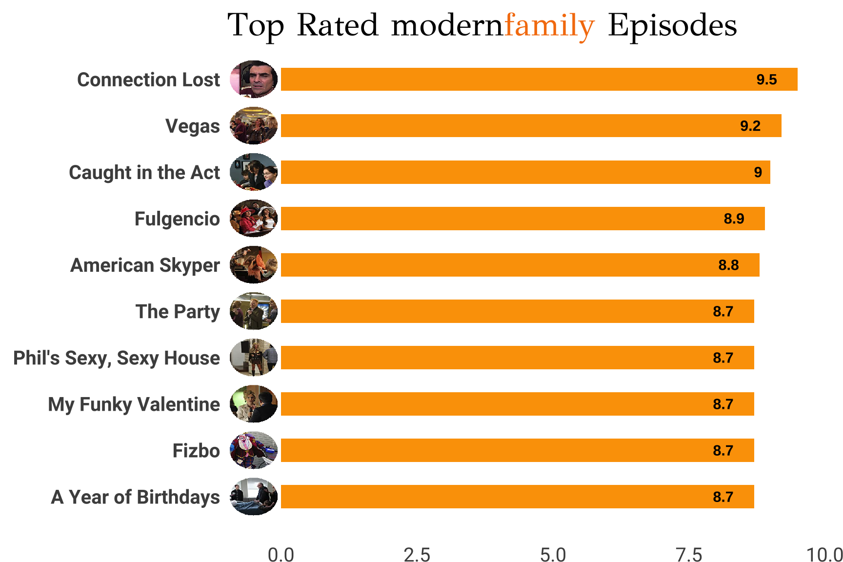
I came across this data on Kaggle and decided to have some fun! I used the data to create a bar plot of the top ten rated episodes of Modern Family.

code

knitr::opts_chunk$set(echo = TRUE, fig.align="center")
knitr::knit_hooks$set(crop = function(...){})
knitr::opts_chunk$set(echo = FALSE, crop=FALSE)

library(tidyverse)
library(ggplot2)
library(ggimage)
library(plotly)
library(magick)
library(cropcircles)
library(geomtextpath)
library(sysfonts)
library(showtext)
library(grid)
library(ggtext)

sysfonts::font_add_google("Roboto", "Roboto")
sysfonts::font_add_google("GFS Didot", "GFS Didot")
showtext::showtext_auto()

modern <- readr::read_csv("~/Desktop/R Projects/modern_familly/modern_family_info.csv")
modern <- as.data.frame(modern)
modern <- modern %>% 
  arrange(desc(Rating))
  
top10 <- modern %>% slice_max(n = 10, order_by = Rating) %>% 
  rename("Image_link" = "Image Link") %>% 
  mutate(Image_link = circle_crop(Image_link))


modernplot <- ggplot(top10, aes(x=reorder(Title, Rating), y=Rating)) +
  geom_col(fill = "#fca103", width = 0.5) +
  coord_flip() +
  geom_text(aes(label= Rating), fontface = "bold", hjust=2, size = 4) +
  geom_image(mapping = aes(y = -0.5, image = Image_link), size = 0.08) +
  theme(axis.title.x = element_blank(),
        axis.title.y = element_blank(),
        axis.ticks = element_blank(),
        axis.text.x = element_text(size = 15, vjust = -3),
        axis.text.y = element_text(size = 15, face = "bold"),
        panel.background = element_blank(),
        text = element_text(family="Roboto"),
        plot.margin=margin(t=10,b=10,l=10,r=14),
        plot.title = element_markdown(size = 25, family = "GFS Didot")) +
  labs(title = "Top Rated modern<b style='color:#f57d0c'>family</b> Episodes")

modernplot